Author and Photographer John Henderson
In Part 1 of this series, we went through some “quick and dirty” calculations that enabled us to choose a suitable size and weight for a semi-scale model that can be expected to sail well. The example we used was a 1:23 model of the J Class yacht Rainbow, and we will continue to use that example in the rest of this series. We will now undertake some more detailed and a bit more extensive calculations to try to get the boat right as built, requiring minimum modifications and fixes after the fact. Not only will this give us a model that is better-constructed, but the radio gear, the ballast, and the sail controls should be more accessible, meaning that they are likely to work better and be more easily and successfully maintained.
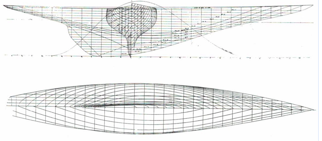
We will begin with displacement calculations. A much-reduced set of lines drawings for the original Rainbow is shown in Fig. 1.
In Part 1 of this series, we used a very much simplified set of lines to explain the roles of the profile, sections, and plan views. The lines drawings for the full-size Rainbow in Fig. 1 are typical of the considerably greater complexity of drawings for an actual boat. Note that the sections drawing has been superimposed on the profile.
As discussed previously, we will probably want our model to have a deeper keel, either by adding a fin-and-bulb or by fairing in some greater depth to the keel profile. For my own 1:23 version of Rainbow, I opted to make the keel about 1.5 in deeper. The easiest way to visualize this (and preserve a pretty profile) is to start by modifying the profile drawing —but note that this means that the sections drawings must also be modified for all sections affected by deepening the keel profile. We would like to preserve the waterline location (for the sake of scale appearance when afloat), but we have added volume below the waterline, which will change the displacement from our “quick and dirty” estimate.
Also, it is common practice for models to have a rudder that is larger than scale size for better handling and control. I followed this practice and made the rudder about 50% larger in area than scale. This also changes the underwater volume.
These changes to the underbody make it desirable to do a new calculation of the displacement. Additionally, I think we should do a more accurate calculation (than the simple division by the cube of the scale factor that we used for quick estimates in Part 1) because that estimate was based on some published weight, which is often inaccurate.
Calculating Displacement
I will review the method of displacement calculation that uses Simpson’s Rule. This is a traditional method that may seem tedious and quaint for folks with access to computer-aided design tools, but it can be done with measuring tools available to everyone and it gives appreciation for the traditional design process. Think “vintage”.
In general, Simpson’s Rule is a method of numeric integration (as in calculus). You can look it up online, but a formulation that is more specific to boat designing can be found in books like Skene’s Elements of Yacht Design. It requires no math skills beyond straightforward arithmetic, but it is time- consuming. It is probably an afternoon of careful work, and you will not be pleased if you discover that you’ve made a mistake part way through.
You begin by measuring the area below the waterline of each half-section on the sections plan of the lines drawings. Simpson’s Rule requires that the sections be evenly spaced and that there be an even number of sections. This explains the numbering of the sections—section #0 is usually located at the forward end of the waterline (not at the bow), and spacing is such that an even-numbered section is located at the aft end of the waterline (#20 in the example I will present). Note that sections in the bow and stern overhangs, which are outside the waterline, are not used in the displacement calculation.
Measuring the areas is the hard part. If you have access to a device called a planimeter, you can trace around each half-section and read the area directly (you probably should do it a couple of times and average the results). I don’t have such a device, so I used a more tedious method: get some engineering graph paper with a reasonably fine grid of squares or make such a grid yourself. Lay this grid of squares over the sections drawings and count the number of squares in each half-section. Since you know the area of each square on your grid, you can compute the area of each section in units of square inches. Be careful, and check each measurement against its neighboring sections for plausibility.
This tabulation of the (below-the-waterline) half- area of each section is the input data to the Simpson’s Rule calculation.
To perform the calculation, you will construct a table as shown in Table 1 below.
- The first column is the section number, from 0 to 20 in our example.
- The second column is the area in square inches of each half-section from the lines drawing, which is what you just measured with the graph paper.
- The third column shows “Simpson’s Multipliers”, which are 1, 2, or 4 in the pattern shown, always starting and ending with 1 .
- The fourth column, labeled “Functions” is the result of multiplying each section half-area by its corresponding Multiplier.
- We’ll talk about the fifth column later when we discuss the Longitudinal Center of Buoyancy (LCB).
- And now, the formula for displacement according to Simpson’s Rule:
Displacement = 2 x [1/3] x [sum of functions of
half-areas] x [inverted scale]2 x [station spacing
interval] x 0.037
where:
- The factor of “2” is because we only measured the half-areas.
- The factor of 1 /3 is per Simpson.
- “Inverted scale” only pertains if we are using drawings that are not full size (as we would for a full-size boat). In our case, using plans that are the size of the actual model, this factor is 1 .
- “0.037” is the density ofsalt water in pounds per cubic inch, because we measured area in square inches. (Salt water density is usually stated as 64 pounds per cubic foot.)
- The calculated units of Displacement are pounds.
The data and associated arithmetic for our 1:23 scale Rainbow example is shown in Table 1.
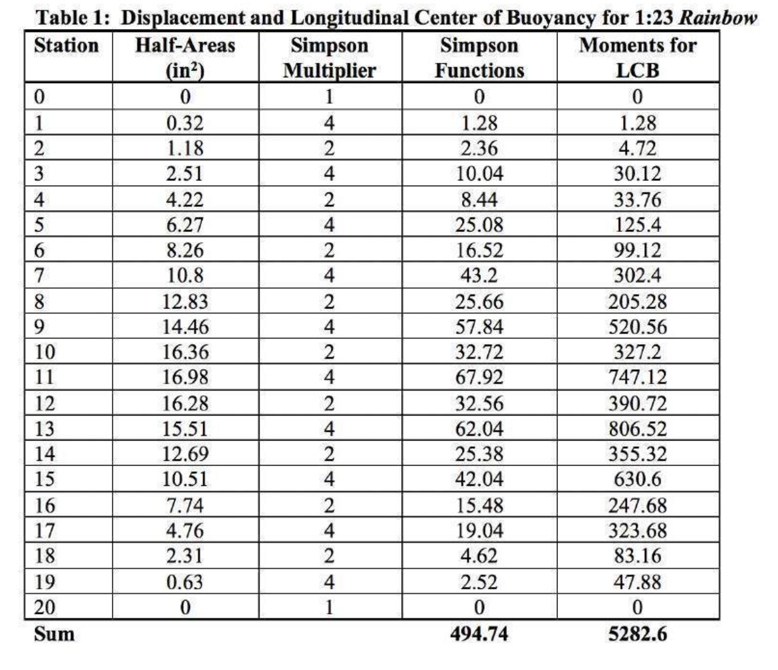
Inserting the sum of Simpson’s Functions into the equation above, and noting that the station spacing on my 1:23 Rainbow example is 2 and 5/32 in (2.156 in) gives
Displacement = 26.3 lb
which is reasonable given the “quick and dirty” estimate of 25.5 lb and noting that we increased the volume of the underbody by adding draft and increasing the size of the rudder. Note that a model of this weight should settle exactly to the waterline. We may want to make the model a bit lighter so that some bottom paint shows at rest.
In fact, we can calculate how much higher the model will float as a function of weight change.
To do this, we first calculate the area of the plane of the waterline in square inches. (Using the plan view of the lines drawings, I did an approximate calculation for the area between each station at the waterline and summed those areas.) Multiplying this area by 1 in gives the volume of water that is 1 in thick in a plane the size of the waterline plane, and we get its weight by multiplying by the density of water (0.037 lb/in3). Sparing you the tedium of yet another table of numbers, I’ll give the result: approximately 3 lb per 1⁄4-in immersion. This means that we can expose a bit of the bottom paint by shaving a couple of pounds off the weight. Or, more usefully and less cosmetically, it shows us the degree of flexibility we have to adjust ballast or control system weight.
Calculating Longitudinal Center of Buoyancy and Center of Gravity
On any reasonable sailing model, the dominant component of total weight is the ballast, and its location fore-and-aft is the major factor in locating the center of gravity of the whole boat. We might want to reserve a small percentage of the total ballast to make trim adjustments if we didn’t get the weight estimates of the rig or the radio quite right, but, basically, we want to get the center of gravity of the ballast in the right place fore-and-aft. Otherwise the boat will trim bow-up or bow-down.
So where must the boat’s center of gravity be located? It must be at the Longitudinal Center of Buoyancy (LCB), which is determined by the shape of the boat’s underbody (the submerged portion of the hull). Calculating the LCB is the purpose of the 5th column in Table 1, called “Moments for LCB”.
The numbers in the LCB Moments column are generated by multiplying Simpson’s Functions (the 4th column) by the number of the station (column #1). This essentially gives the “leverage” that the buoyancy of each station provides relative to station 0 (the forward end of the waterline). Those moments are summed, as given at the bottom of column 5. The sum of these moments is then divided by the sum of Simpson’s Functions, to give:
5282.6 / 494.74 = 10.68
This means that the LCB is located 10.68 stations aft of station 0, which, for the station spacing in this example model, is 23.03 in.
So, if we suspend the boat (in the air) from this point, we must arrange the ballast and other gear so that it balances level. Ballast has the dominant effect, but it would be good to locate the radio gear in its approximate position (especially the battery and any big servos) and to place 1.5–2 lb at the mast location (calculated below) to simulate the rig weight.
Mast Location and Center of Effort
If we make changes to either the rig or the underbody—and we have made the case for such changes in all of the previous discussions—then we need to re-visit the helm balance. When sailing on a reasonably close-hauled course, the boat should want to continue sailing in a straight line or—as I prefer because it is what I like in a full-size boat—the boat should have a slight tendency to round up to weather. This is called “weather helm”. The boat should never want to head off away from the wind (called “lee helm”) because correcting this with the rudder introduces drag and a sailing angle change that actually reduce progress to windward. Proper helm balance requires the right relationship between the Center of Effort of the sail plan and the Center of Lateral Resistance of the hull underbody.
The locations of both of these Centers change dynamically with sail trim, sailing angle, and heel angle, but those dynamic changes are beyond the scope of this article. We can, however, get pretty close by considering the problem statically, and I think this is the traditional design technique. Both Centers can be thought of as the single points where all of the respective forces of wind on the sails and water on the underbody could be centered—analogous to the Center of Gravity for weight.
There is a simple and non-technical procedure for locating the Center of Lateral Resistance (CLR) of the underbody:
- Trace the area of the profile view that is below the waterline onto a piece of light and stiff material, like cardboard.
- Balance this cardboard cutout on a ruler edge that is perpendicular to the waterline. The fore-aft CLR is at this balance point. (You only need the fore-aft location for this exercise: the vertical location does not matter.)
If you are planning to add a fin-and-bulb keel, then the CLR of this added keel should be at about the same position as the original CLR.
Locating the Center of Effort (CE) of the sail plan is only slightly more complicated.
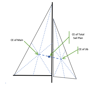
With reference to Fig. 2:
- Create an accurate drawing of the sail plan, including main and jib. This could be much smaller than your actual model, but it must be scaled from your model plans.
- For each sail, draw lines from each corner (tack, clew, head) to the center of the opposite edge of the sail. The CE for that sail is located where these lines meet.
- The CE for the entire sail plan is located on a line that joins the individual Centers of Effort, and its exact location must be “weighted” by the relative areas of the two sails. Here we’ll compute the distance by which the total CE is aft of the mast, which is:
{[area of main] x [dist. of its CE aft of mast] – [area of jib] x [dist. of its CE forward of mast]} / {total sail area}
The reason for doing all this is to determine the location of the mast. Go through the same exercise on the plans for the original boat and compare your model boat’s CE and CLR locations with those of the original boat. It is likely that the CLR will have changed only very slightly, unless you have made the underbody substantially different. The CE of the sail plan may have changed much more (recall that we made the case for a significant reduction in the scale sail area). If the CLR is not much changed, then you must (re)locate the mast so that the CE of the sail plan (not the mast location) matches the original CE. If the mast must move to a non-scale position, that is the consequence of making a (semi) scale model that sails well.
In the event that the CLR has also moved substantially, then you must locate the sail plan relative to this new CLR. This is tricky, and I believe that the result obtained by using these static measurements will be only approximate. I have read many opinions on the proper relative locations of the CE vs the CLR, ranging from “CE directly above CLR” (which I believe to be wrong) to “CE forward of the CLR by ~17% of the waterline length” (which I believe more likely to be correct).
The reason to try to get this right is to “balance” the helm with a slight amount of weather helm, which is what causes the boat to want to “round up” into the wind. When the boat is completely upright, the turning forces on the hull are balanced, but when the boat heels, the heeled waterline is not symmetric—the leeward side presents a more rounded entry than the heeled windward side, and this tends to turn the boat into the wind. Much more important, however, is the effect of heeling on the sail forces. When the boat heels, the driving force of the sail shifts from being more-or-less directly above the hull to being off to the leeward side by an amount that depends on the heel angle. This offset force produces a torque that turns the boat to weather. (If you doubt this reasoning, consider how a sailboard steers.)
To counteract this force turning the boat to weather too strongly, we can move the CE of the sail plan forward, which would tend to steer the boat to leeward. The problem is: “How much forward and at what heel angle do we make this calculation?” Hence the “trickiness” and uncertainty. I suggest that the mast be located so that the CE is forward of the CLR by 15 to 17% of the length of the waterline. I would also suggest that you construct the mast step and chain plates in a way that allows this location to be adjusted. Even full-size boats with professional designers often end up moving the mast or changing mast rake after sailing trials reveal the necessity.
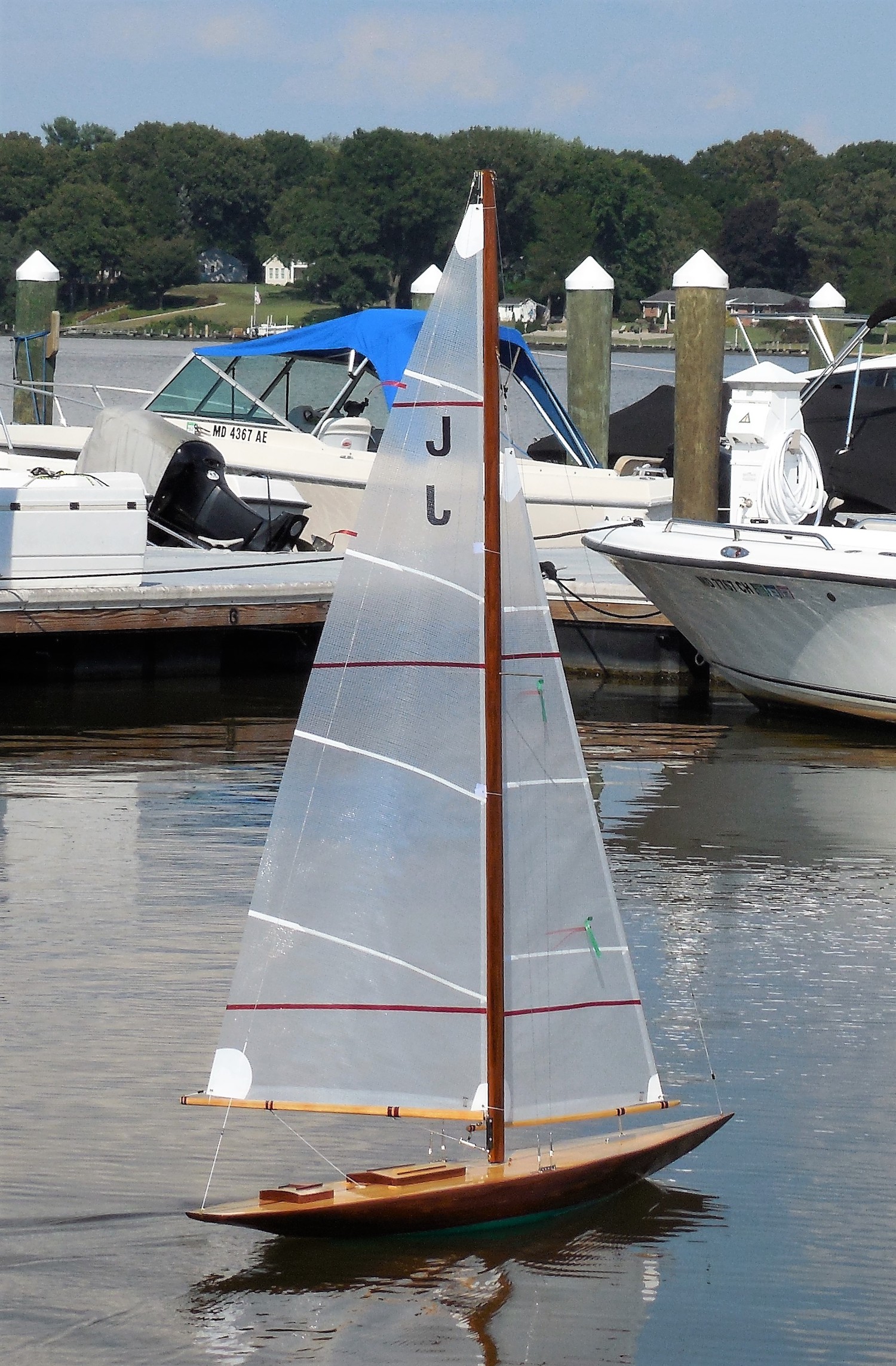
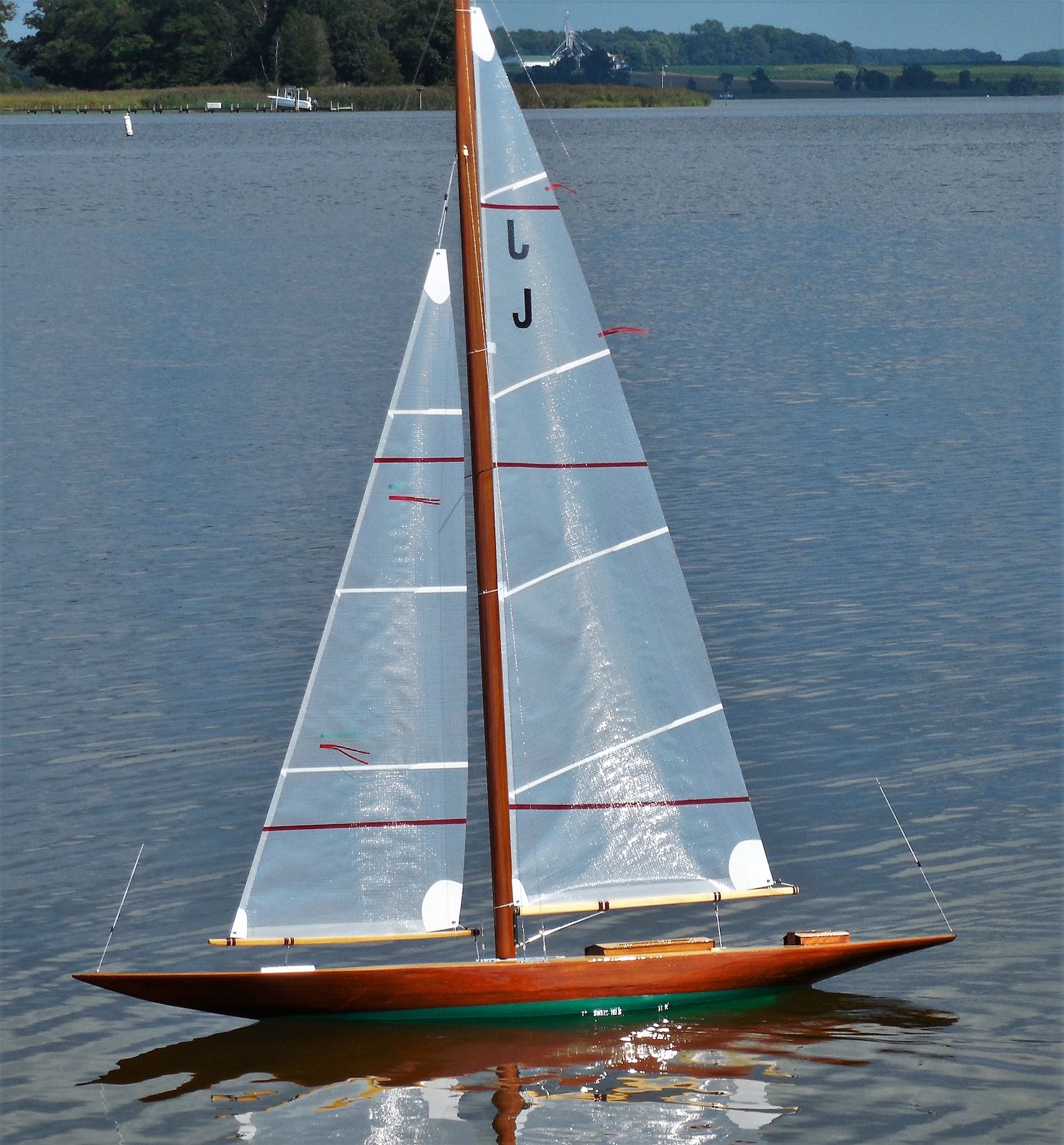
Figures 3 and 4 show the model on its initial sail, built according to the processes above and unmodified from “as built”. The conditions were light air and very sheltered water—also quite crowded and small, as the photos show. The boat was deliberately launched at about 3 lb below the weight calculated to float it at its exact waterline.
The amount of waterline showing was very close to the predicted 1⁄4 in. The helm balance was pretty neutral, with slight weather helm on a reach or if a gust came through. I intend to experiment with some added ballast and moving the mast aft ~1⁄2 in.
These calculations and thought processes form a good basis for planning and building a sailing scale model of a real boat. There are many more calculations that designers make as they evaluate the performance of their designs, but our exercise is not about undertaking an original design. For whatever reason, we will choose a design with its associated performance characteristics, and we hope to make a reasonable scale reproduction, modified only to the extent necessary to make it sail well at our chosen scale. Ina future article, we will go through the process of building the model we have been using as an example, solving some of the practical issues that are unique to sailing models.